Comparing energy and exergy of multiple effect freeze desalination to MEE MSF RO – npj Clean Water

Design of MEFD

Several terms have been used in the literature instead of the SSDE and the SSRR. During crystallization, a certain amount of salt is rejected from the ice crystal, and a portion of the salt stays between the crystal boundaries. Therefore, the single-stage desalination efficiency (SSDE) is defined as the ratio of the salt concentration of the ice to the incoming solute. Other terms such as desalination rate^14,15, removal efficiency⁶, and salt removal efficiency^16,17 are also used interchangeably with SSDE. Most of the articles in the FD are currently focused on improving the SSDE. However, there is another very important criterion for making FD viable for commercial use, the SSRR. Similarly, the SSRR is defined as the ratio of the mass of the ice produced to the total mass of the incoming solute. Other similar terms such as solid fraction¹⁴, ice ratio³, fraction of solid phase², ice yield rate¹⁸, ice mass fraction¹⁹, and recovery ratio⁸ are also used to represent the SSRR.

It is important to distinguish between the terms “single-stage” and “total” when comparing literature data. While some studies use them interchangeably, a clear distinction is made between them. “Single-stage” is used to refer to the efficiency and the recovery rate in only one single stage of FD, and “total” refers to the efficiency and recovery rate for all effects of MEFD combined. For example, the SSDE may be only 50%, but the total desalination efficiency may be 95% or higher.

In MEFD, each stage is a vessel where feed water freezes and separates into ice and brine. The ice still contains some salt, depending on the SSDE. To purify the ice, it must move to the next effect until the desired limit is reached. On the brine side, FD is resistant to scaling and fouling so it may not require chemical pretreatments. Additionally, the low temperature makes it resistant to corrosion. The maximum brine limit for MEE, MSF, and RO is around 70,000 ppm^20,21,22. However, hybrid methods such as nanofiltration can improve the maximum brine concentration. These limits are not fixed and depend on the temperature and types of solids in the feed. Increasing the limits increases the maintenance and operational costs.

The FD technology is still in its early stages, and more research is needed to determine the highest limit of brine concentration. However, FD shows promise for higher limits of brine concentration, up to 200,000 ppm²³. To be conservative, the maximum reject brine concentration is assumed to be 120,000 ppm. The maximum brine concentration affects the total recovery rate, but the goal of the current study is not to present a ZLD technique with a total recovery rate of 100%.

The feed concentration is considered to be 40,000 ppm. Figure 1 shows the schematic for each stage of the MEFD. \(x\) represents the salt concentration in ppm. The feed is injected into the system and goes through a batch process, including freezing, separation, melting, and washing. The concentration of the salt in the reduced salt water is checked. If the concentration of the salt water is less than 900 ppm, it is considered fresh water and no further processing is required. The limit for considering fresh water is debatable, with some considering 500 ppm as the proper edible limit for potable water. For the purpose of introducing the MEFD in the current study, 900 ppm is considered as the fresh water limit. The 900 ppm limit is for the outcome of only one stage, and therefore, mixing the potable water from multiple effects, depending on the process flow, reduces this number to even lower concentrations, as shown later in the text.

In the current study, a distinction is made between the effect and the stage. An effect is comprised of several stages of desalination. If the reduced-salt-water salt concentration is more than 900 ppm, it is sent to a new stage in a new effect. Each effect is comprised of one or more stages and each stage has a certain incoming feed concentration. Each effect may have several incoming feed concentrations and is directed to different stages within the effect. The final fresh water product is comprised of multiple water amounts with different salt concentrations of lower than 900 ppm. Therefore, after mixing all of the products, the final salt concentration is lower than 900 ppm and can be calculated.

The brine salt concentration is checked after each effect. If the brine salt concentration is more than 120,000 ppm, it is considered reject water. If the brine salt concentration is less than 120,000 ppm, the volume of the brine is assessed. If the volume of the brine is too low (1% in the current study), it is considered reject water as well. This small amount of water is rejected regardless of the salt content. Otherwise, the brine is sent to a new stage in a new effect. The 1% criterion is subjective and serves as an example of how the system operates. This number may be altered by the MEFD system designer.

The output of each stage is two streams of water with different salt concentrations, as shown in Fig. 1. The next effect must have at least two separate stages to accommodate the two different feed concentrations. Feed waters with similar salt concentrations may be combined into one stage, as long as they are compatible.

Figure 2 illustrates the schematic of an MEFD, while additional specifics of the single-stage FD unit are outlined in Fig. 3. There is only one feed to the first effect, which contains 40,000 ppm of salt, and one stage is sufficient for processing the feed. The first effect has two output concentrations: reduced salt and brine. If the reduced salt and the brine meet the previously described conditions, they are directed to the second effect. Since the salt concentrations are different, two stages are required within the second effect to process the outgoing stream from the first effect. The process continues to the third effect and so on, with the number of stages in each effect depending on the number of outputs from the previous effect that require further processing. The process flow is complex and highly dependent on the SSDE and the SSRR. In the current study, several different SSDEs and SSRRs are assumed to design the process flow.

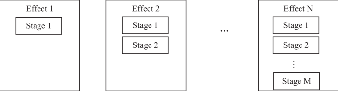
Each effect contains several stages.

The components are labeled as follows. “L#”s represent sensors. “A” denotes the evaporator unit. “B” refers to the FD main chamber unit. “C” indicates the compressor for the refrigeration unit. “D” signifies the auxiliary condenser unit #1 for recovering cold brine energy. “E” represents the main condenser unit for recovering ice energy. “F” is the auxiliary condenser unit #2 for controlling the final refrigerant temperature due to uncontrolled or ambient condition variations. “G” indicates the expansion valve. The flow directions of the refrigerant are numbered 1–6. “H” represents the brine flow after energy recovery in the auxiliary condenser unit #1, which proceeds to the subsequent stage. “J” signifies the ice flow after melting and energy recovery in the main condenser unit, which continues to the next stage. “K” denotes the primary control unit.

The current design, explained in more detail in ref. ²⁴, introduces several notable innovations. Firstly, a comprehensive methodology for designing an MEFD system is established. Secondly, several new designs are presented, some of which are highly complex and have not been explored experimentally or theoretically before. These designs incorporate up to hundreds of stages and effects, necessitated by low values of SSDE and SSRR.

Additionally, the current study marks the first instance in which the total energy consumption across all stages and effects of an MEFD is meticulously calculated. Another significant innovation is the varying energy usage across different stages and effects, which arises from changes in brine concentration affecting the freezing point. This variability adds further complexity to the energy usage calculations.

Experimental setup

To make better initial assumptions, an experimental setup is designed to extract the SSDE and the SSRR for a baseline measurement. No improvements to the baseline are intended at this point. The experimental tests are performed solely to establish baseline numbers for the process design.

There are numerous methods to choose from for an experimental setup. The goal is to perform baseline tests, so the most straightforward approach is selected. Figure 4 illustrates the experimental setup for FD, where the solution is frozen from top to bottom. Stirring methods and post-washing techniques are intentionally avoided to assess the ice quality in its natural state. As per literature⁶, the ice quality for top-to-bottom freeze has better quality, and therefore, freezing is conducted from top to the bottom. The coolant plate temperature is maintained at a constant −9 °C, and the solute content is insulated all around. As the ice forms from the top and progresses downward, more solute content freezes, causing the salt to be rejected and concentrated in the remaining solution. This test is repeated multiple times to obtain various amounts of ice. The concentrated solute is then separated from the original content, and the ice content is measured. After melting the ice, the salt concentration of the resulting water is measured.

The container, with a diameter of 9.5 cm and a height of 6.5 cm, is well insulated all around to enforce top-to-bottom freezing. Once the liquid is in the container, the freezing process starts from the top and gradually progresses towards the bottom, resulting in the formation of ice layers. After the ice is fully formed, it is carefully removed from the container. The removed ice is then melted down to a lab-controlled temperature and measured.

The configuration depicted in Fig. 5 is tailored for temperature supervision, comprising an Arduino Uno, two temperature sensors, a timer, a display, and an SD card module for data storage. Following the production of each ice batch, the brine is separated via the bottom valve and quantified, while the remaining ice content is transferred to a separate receptacle. The ice is quantified, melted, and then subjected to salt content analysis using two techniques: initially, at a controlled 24 °C lab temperature, the salt content is assessed with a METROHM 660 conductometer. Subsequently, both the melted ice and brine undergo complete evaporation to accurately determine the residual salt content.

Left: Control system; Right: Single temperature sensor adjacent to the evaporator.

By establishing the initial salt content in the feed, the salt content of both the melted ice and remaining brine has now been determined. With knowledge of the mass of melted ice and brine, the single-stage recovery rate can be computed. Furthermore, knowing the salt content of both components allows for the measurement of SSDE. These results are replicated multiple times and presented in Fig. 6.

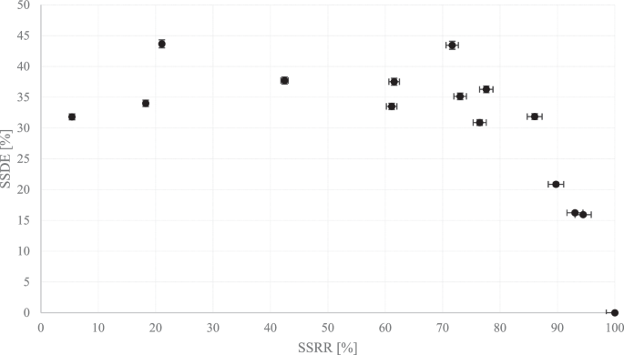
No stirring or post-treatments applied to ice content; an SSRR below 75% is optimal, yielding the highest SSDEs.

It is important to note that this may be the first instance in which SSDE and SSRR are clearly, meticulously, and methodologically plotted against each other as baseline values, without the introduction of any additional parameters such as post-washing techniques.

The results, displayed in Fig. 6, indicate that higher SSDEs are being sought at higher SSRRs. For SSRRs ranging from 20% to 80%, the SSDEs range from 35% to 45%. Both the SSDE and SSRR can be further improved through post-treatment. To illustrate the importance of the recovery rate in the process design for an MEFD, the process design begins with an SSDE of 50% at an SSRR of 50%.

The decision to opt for 50% in both SSDE and SSRR is discretionary and hinges on the objectives of the MEFD designer. The selection of these values was influenced by foundational data gleaned from Fig. 6, along with potential enhancements that could be implemented with relative ease. Notably, as will be elucidated later, a process flow incorporating 50% SSDE and SSRR is notably intricate, and reducing these figures would significantly heighten the analytical complexity. To illustrate, a configuration featuring 50% SSDE and SSRR entails ~40 effects, each comprising multiple stages. The energy computation for this extensive setup poses considerable challenges. Hence, the process is initiated with 50% SSDE and SSRR, with intention to increment these values subsequently.

Figure 7 illustrates the process flow for a freezing plant with a 50% SSDE and 50% SSRR. The initial feed salt content is assumed to be 40,000 ppm and is shown on the left side of the process. Since all of the salt content cannot be rejected within a single effect, multiple effects of desalination are required to reach the desired freshwater level. Within each effect, there may be one or more stages of desalination. Within each stage of the desalination, the vessel freezes the incoming solute, then the ice is removed from the vessel and melts down in a second vessel and the energy is recycled as much as possible by reducing the condenser temperature and hence improving the cycle COP.

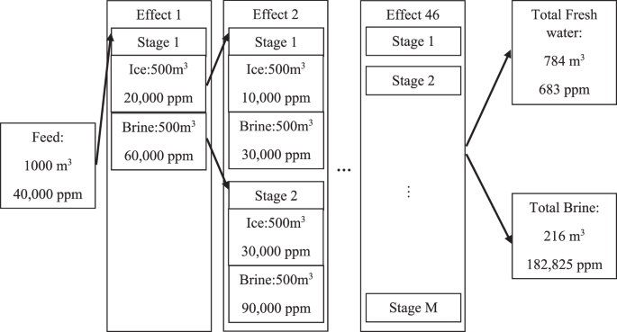
This process flow utilizes 46 effects of freeze desalination to achieve a total recovery rate of 78%.

The melted ice has a lower salt content compared to the original feed. The molten ice goes through the next effect and gets further purified. This process continues until the ice is considered acceptable for fresh water. For simplicity, the criterion for accepting the purified ice is considered to be 900 ppm within each stage, which is somewhat higher than the potable water standards. The final product, however, is expected to have less than 900 ppm of salt content since it is a mixture of the final products of all the effects. For instance, as shown in Fig. 7, the final product of all the effects is 784 m³ of fresh water (total recovery rate of 78.4%) at 683 ppm. The aggregated final product purity is illustrated in Fig. 8, which demonstrates that the final product purity ranges from 300 to 700 ppm, despite the single-stage purity criterion being set at 900 ppm.

Although the single-stage product water criterion is 900 ppm, the final aggregated product is below 700 ppm due to mixing from different effects.

During each stage and the freezing process, the extra salt content of the ice gets rejected to the rest of the solute, creating a highly concentrated solute. The highly concentrated solute may or may not be further desalinated based on the designer’s goals. For better comparison between different design scenarios, a rejection criterion of 120,000 ppm is considered for the concentrated solute. Another rejection criterion in the current study is when the solute volume is less than 1% of the original incoming water.

Both of the criteria for acceptance or rejection of the concentrated solute are subjective and depend on the designer and the economies of scale. Assuming 1000 m³ of feed water, half of the incoming solute freezes since the SSRR is 50%. The other half of the incoming solute, the concentrated solute, should contain more salt content. The salt content of the ice portion is 20,000 ppm since the SSDE is 50%. The rejected salt content of the ice moves to the concentrated solute, and the solute contains 60,000 ppm. The ice content has to be desalinated again and is directed to the first stage of the second effect. The same process is repeated in the stage 1 of the effect 2 and continues until the fresh water criterion of 900 ppm is satisfied and does not require any further desalination.

On the brine side of the first effect, the brine volume is 500 m³ and the brine salt content is 60,000 ppm, satisfying the recycling criteria and has to be recycled. The brine is directed to the second stage of the second effect and the same process repeats. The process schematic shown in Fig. 7 is only a summary of the full schematic since the full schematic, which is quite complex and does not fit within a small figure print.

After 6 effects of desalination of the ice, 1.6% of the incoming solute ends up being fresh water. To obtain more fresh water, the concentrated solutes from each stage within each effect should also be desalinated multiple times. The process repeats as many times as needed until one of the acceptance or rejection criteria is satisfied.

The number of effects required for desalination depends on both the SSRR and the SSDE. For instance, with an SSRR and SSDE of 50%, it takes 46 effects of desalination to recover 78% of the incoming water. The salt concentration within the ice and the brine are formulated within each stage of the desalination. The salt concentration within the ice for each stage can be calculated as:

in which \({C}_{{ice}}\) is the average concentration of the salt in the frozen portion of the mixture (ppm), \({C}_{{incoming\; mixture\; to\; the\; stage}}\) is the average concentration of the salt in the feed water to the desalination stage (ppm), and \(\eta\) is the SSDE (0–1). For instance, if the incoming salt content of the solute to the first stage of the first effect is 40,000 ppm, the salt content within the ice after the first stage of the first effect can be calculated to be 20,000 ppm with the SSDE of 50% (\(\eta\) = 0.5). The salt content of the concentrated solute can be calculated using Eq. (2),

in which \(R\) is the SSRR (0–1) equivalent to the volume percentage of the ice divided by the total incoming mixture within each stage. The salt content of the concentrated solute after the first stage is therefore calculated to be 60,000 ppm for the SSRR of 50% (\(R\) = 0.5).

The MEFD is designed for different SSRRs and SSDEs. The procedure is repeated for the SSRR of 50% with the SSDEs of 60%, 70%, 80%, 90%, and 100%. Then the procedure is repeated for the SSDE of 50% with the SSRRs of 60%, 70%, 80%, 90%, and 99.9%. Finally, the procedure is repeated for equal SSDEs and SSRRs of 60%, 70%, 80%, 90%, and 100%. The number of effects required for each stage is calculated and plotted in Fig. 9.

a The number of process effects required with different SSDEs is shown on the left axis, with a fixed SSRR of 50%. b The number of process effects required with different SSRRs is shown on the right axis, with a fixed SSDE of 50%. c The number of process effects required with varying SSDEs and SSRRs is shown. Both the SSDEs and the SSRRs are altered together.

Figure 9 illustrates the number of effects required for an MEFD with different numbers of SSDEs and SSRRs. Figure 9a shows the effect of the SSDE with a fixed SSRR of 50%. The number of process effects in an MEFD is directly related to the capital and indirectly related to the operational cost of the desalination plant. Improving the SSDE is critical in reducing the number process effects and hence the capital costs. For instance, reducing a plant size from 40 effects to 10 effects is probably reducing the capital costs by at least 75%. Figure 9b displays the effect of the SSRR with a fixed SSDE of 50%. Improving the SSDE is more critical than improving the SSRR, but improving the SSRR is important in designing a low capital cost MEFD plant. Figure 9c displays the effect of improving both the SSDE and the SSRR together, which leads to a drastic improvement over improving just one factor. For instance, for the SSDE of 80% and the SSRR of 50%, 16 effects are required. For the SSRR of 80% and the SSDE of 50%, 24 effects are required. By improving both the SSDE and the SSRR to 80%, only 10 effects are required to complete the task.

In Fig. 10, the relationship between the number of effects and SSDE/SSRR is depicted. Although only six data points are utilized to construct this graph, it should be noted that extracting data for even these six points is a labor-intensive endeavor. Notably, certain data points, particularly those corresponding to lower SSDE/SSRR values, involve dozens of effects with multiple stages within each effect, contributing to a substantial background in the dataset.

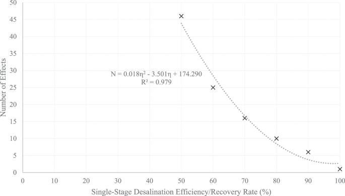
As SSDE/SSRR increases, the required number of effects decreases significantly.

A second-order polynomial can be used to approximate the relationship between the number of effects and the SSDE/SSRR in Fig. 10:

where \(N\) represents the number of effects and \(\eta =R\) represents the SSDE/SSRR.

Equation 3 demonstrates a significant second-order effect on the number of effects in the MEFD process when the SSDE/SSRR is modified.

Energy comparison with RO/MEE/MSF

To provide clarity, the feed concentration for RO, MEE, MSF, and MEFD is set at 40,000 ppm. The permeate/distillate concentration is maintained below 500 ppm except for MEFD. In the case of MEFD, given its intricate design, the single-stage product concentration is stipulated to be under 900 ppm, with the overall MEFD concentration consistently falling within the range of 500–900 ppm, varying depending on the specific MEFD setup and the number of effects involved. The total number of effects/stages in RO, MEE, MSF, and MEFD varies significantly and plays a crucial role in comparative evaluations. The significance of energy recovery in MEFD becomes evident in the upcoming comparison. The energy recovery in MEFD is intertwined with the COP of the single-stage FD designs. It will be demonstrated later that energy recovery in MEFD is achieved through condenser temperature reduction. By utilizing literature data, comparisons are conducted across various COP values, thereby integrating energy recovery into the COP calculations.

An MEFD process is expected to be more efficient and effective than a single-effect FD due to its ability to desalinate water to a much higher level and achieve a higher recovery rate. The latent heat of solidification of water, which is approximately 334 kJ/kg²⁵, is significantly lower than the latent heat of water vaporization, which is approximately 2260 kJ/kg²⁶. From the perspective of the energy usage, the freeze techniques are believed to potentially use much less energy than distillation^6,27. This statement is evaluated in more detail.

In the context of thermal desalination techniques, multiple effects of distillation and/or flashing are designed to be more energy-efficient than single-stage distillation techniques. This can be observed in the energy requirements per unit of distillate for MEE and MSF processes. The heating energy required per kg of the distillate, using an MEE with 10 and 20 effects is calculated from Eq. (4)²⁸:

and are approximately 319 and 177 kJ, respectively. In Eq. 4, \({\dot{Q}}_{H,{MEE}}\) is the required heating energy, \({\dot{m}}_{D}\) is the distillate mass flow rate, \({\Delta h}_{v,{T}_{v,{m}}}\) is the latent heat of vaporization at the mean temperature of the effects, and \(N\) is the number of effects. It is also shown that with the same number of effects, an MEE always consumes less energy compared to an MSF²⁸.

A major distinction exists between the energy usage of FD and MEE/MSF techniques. The primary energy source for FD is high-grade energy (electricity), while MEE/MSF rely on low-grade energy in the form of heat at lower temperatures. To provide the necessary cooling energy, FD requires a vapor compression cycle with a certain COP. Some of these scenarios are detailed in Fig. 11. For example, using a COP of 3, only 111 kJ of electricity is needed to provide 334 kJ of cooling energy. A power plant with 35–60% thermal efficiency uses 317–185 kJ of heating energy to provide 111 kJ of electricity. Similarly, a vapor compression cycle with a COP of 12, requires only 28 kJ of electricity, which corresponds to 80–47 kJ of heating energy from the power plant. In comparison, a single effect/stage of FD initially seems to use approximately 47–317 kJ of heating energy per kg of distillate, which is comparable to 10–20 effects of MEE. However, these calculations assume that a single-stage FD has almost perfect desalination efficiency and recovery rate, which is not the case in reality.

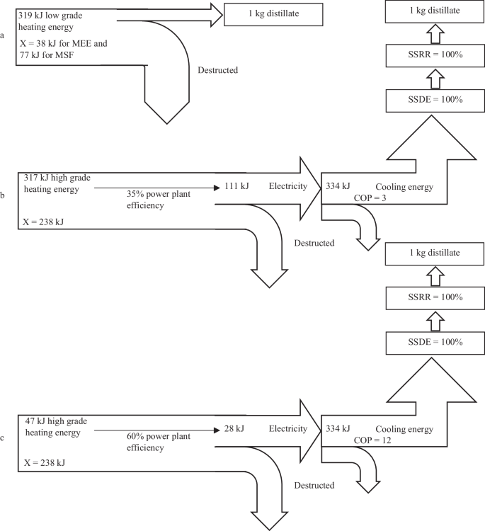
a MEE and MSF, b MEFD with SSDE/SSRR = 100%, COP = 3, and a power plant efficiency of 35%, c MEFD with SSDE/SSRR = 100%, COP = 12, and a power plant efficiency of 60%. While this graph appears promising, a thorough examination of the impact of SSDE and SSRR is warranted.

The grade of the 47–317 kJ of heating energy used in a power plant to produce 28–111 kJ of electricity is still higher than the grade of the 177–319 kJ of heating energy used in 20–10 effects of MEE/MSF plants. The heating energy grade consumed in a power plant to produce the electrical energy used for the FD is much higher than the lower grade heating energy consumed in the MEE/MSF plants. Therefore, an exergy case study is required for a fairer comparison.

The grade of 47–317 kJ of the heating energy used in a power plant to produce the required electrical energy for the MEFD depends on the high and low temperatures of the power plant that produces the electricity. For example, a power plant with a high temperature of \({T}_{H}=1200{K}\) and a low temperature of \({T}_{L}=300{K}\) has a reversible efficiency calculated as:

In this case, the power produced by the reversible heat engine and the exergy is 35–238 kJ.

The exergy of the 177–319 kJ of the heating energy used in 20–10 effects of the MEE/MSF is significantly lower compared to the exergy used in a power plant to produce the required electrical energy for the MEFD. The heating required for an MEE/MSF may be extracted from the low-pressure steam turbine. The temperature of the MSF plants is typically higher and around 120 °C while the temperature of the MEE plants is typically lower and around 70 °C. Therefore, the high temperature in an MSF/MEE plant is considered to be around \({T}_{H}=393{K}\) and the low temperature is \({T}_{L}=300{K}\). The reversible efficiency for this temperature range is 0.24, resulting in an exergy of 42–77 kJ for the 177–319 kJ of heating energy used in 20–10 effects of the MEE/MSF plants. Therefore, the exergy of the heating energy used in the power plant for the MEFD is much higher than the exergy of the heating energy used in the MEE/MSF plants, highlighting the need for an exergy analysis to provide a more accurate comparison between the desalination processes.

A single-stage FD appears to use a similar or higher amount of exergy compared to 20–10 effects of the MEE/MSF, despite their initial energy-wise comparability. A more precise calculation of the energy requirements for the FD compared to the MEE/MSF seems feasible. One crucial aspect in reducing the energy requirement for the MEFD is through recycling the cold energy at the end of each stage.

Energy recovery in a single stage could involve lowering seawater temperature without melting ice or solidifying seawater, as the solidification temperature of seawater is slightly lower than that of melted ice. The cleanliness and temperature differences between melted ice and seawater, influenced by SSDE, significantly impact design considerations. Enhancing FD efficiency can involve improving the COP by introducing ice to the condenser and minimizing the condenser temperature towards the evaporator temperature. Another approach is to maintain fixed SSDE and SSRR values while designing the total number of effects/stages and transferring ice from initial to final stages while ensuring consistent mass flow rates throughout. While these scenarios are not detailed in this paper, calculations, and designs have been conducted exploring these concepts. The complexity of MEFD energy recovery may limit the ability to fully address all scenarios within the current study and a range of COPs is only being considered. As the COPs are improved, more energy is recovered.

The cold energy at the end of each stage of an FD can be utilized to decrease the condenser temperature of the vapor compression cycle, thereby increasing its COP. The calculations introduce a wide range of COPs from 3 to 12 to account for the possible energy recycling potential during the MEFD. The design of an MEFD is explained in the previous section, and the energy used in each effect depends on the SSRR and the SSDE of each stage. The efficiency of each stage affects the amount of subcooling required for freezing the salted water, which is turn affects the energy requirement. For instance, a higher SSDE removes more salt from the partially desalinated portion of the salted water and hence the subcooling is affected. The recovery rate influences the amount of material being frozen and, consequently, the required freezing energy. The energy required for freezing the salted water depends on the salt content, which varies within each stage. In general, the energy required for freezing the salted water per \({m}^{3}\) of the incoming water to the stage can be calculated as:

where \({T}_{{ini}}\) is the water temperature before the freezing process, \({H}_{{fi}}\) is the latent heat of solidification, \({c}_{p}\) is the specific heat capacity of water, \(i\) is the van’t Hoff’s factor relative to the number of ion particles which is 2 for NaCl^29,30,31,32, \({K}_{f}\) is the cryoscopic constant (which is \(1.86{Kkg}/{mol}\) for water^29,30,31,32), \(\rho\) is the density, and \({\rm M}\) is the molar mass of NaCl.

In Eq. 6, the first bracket represents the amount of energy required to reduce the temperature of the \(R\) portion of the salted water from the initial conditions to the final conditions within one single stage of the MEFD. The second bracket represents the amount of energy required to reduce the temperature of the rest of the content of the MEFD stage (the unfrozen portion) from the initial conditions to the final conditions within one single stage of the MEFD.

The first term in each bracket in Eq. 6 represents the required cooling to reduce the temperature of the stage from the initial temperature to 0 °C. In the current study, the initial temperature in considered to be 30 °C. The last term in each bracket is the subzero cooling required to freeze a certain concentration of the water. The second term within the first bracket in Eq. 6 is the energy required to overcome the latent heat of solidification for the frozen portion of each stage.

The energy required for freezing as calculated from Eq. 6, can be further modified to account for extra energy needed to stabilize the ice content³⁰. Additionally, more energy is required for washing, pumping, stirring, and other utilities used for the FD. In this analysis, a conservative approach is taken by not calculating the freezing energy required for stabilizing the ice and the utility electrical usage, as it will later be shows that even the conservative energy calculation for the FD demonstrates significant energy usage.

In an MEFD, there are multiple stages within each effect, and the incoming and outgoing masses and concentrations for each stage depend on the SSDE and the SSRR. The energy calculations are performed for an MEFD with varying amounts of \(\eta\) and \(R\) for each of the single stages within the design, and the results are added up. For example, for \(\eta =R=50 \%\), the energy calculations for 173 stages within 46 effects are extracted and added up to calculate the total required cooling energy.

The total required specific cooling energy, which is the required cooling energy divided by the \({m}^{3}\) of the desalted water, is shown in Fig. 12 for several different design scenarios. The specific cooling energies for an MEFD vary from 8000 to 459 \({MJ}/{m}^{3}\). This is significantly higher than the previous calculation of 334 \({kJ}/{kg}\), which only accounted for the latent heat of solidification and did not consider the cooling energy required for reducing the temperature of the salted water to zero and the subzero cooling. Additionally, the previous calculation did not account for multiple effects. Therefore, a more complicated calculation reveals much higher energy usage for the FD than initially expected.

As SSDE/SSRR increases, the required specific cooling energy decreases significantly.

The specific cooling energy required for an MEFD is divided per number of effects of the MEFD and presented in Fig. 13. The results show that 100-459 \({MJ}/{m}^{3}\) of energy is needed for each individual effect of an MEFD. While lower \(\eta\) and \(R\) values require less energy per effect, they only necessitate a higher number of effects (as shown in Figs. 9–10 and 12), resulting in significantly higher total calculated cooling energies. Therefore, operating with higher \(\eta\) and \(R\) values is more favorable due to the less complex design and, as later demonstrated, the lower total energy usage, even though the required energy per effect is higher.

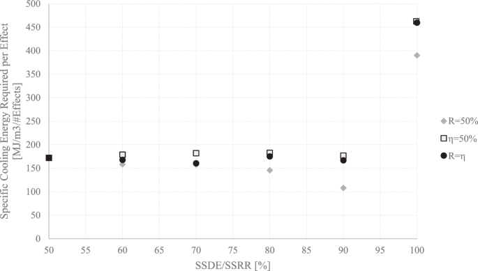
As the SSDE/SSRR increases, more cooling energy is required per number of effects. This is due to the reduction in the number of effects, which may be more favorable as the complexity of the design heavily reduces.

The specific cooling energy required for an MEFD cannot be directly compared to desalination techniques. The electrical energy required for providing a certain cooling energy from a vapor compression cycle depends on the COP of the cycle. Achieving a higher COP such as 12, by recycling the energy of the molten material in the condenser of the FD is also reported to be possible^3,33.

To demonstrate the highest and possibly close to the lowest limits of the electrical energy required for running an MEFD, both COPs of 3 and 12 have been used, and the specific electrical consumption is plotted in Fig. 14. An MEFD with the ideal and probably almost impossible case of \(\eta =100 \%\) and \(R=99.9 \%\), uses \(38.3{MJ}/{m}^{3}\) which is close to the current RO electrical consumption for seawater. Since both the RO and the MEFD use electricity as the input energy, no further exergy analysis is required, and the comparison is fair and final.

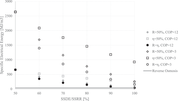
The electrical energy depends on the COP of the vapor compression cycle. In this figure, the specific cooling energy for the vapor compression cycles with COP = 3 and COP = 12 are determined.

The RO seems to be using less energy (~21–72 \({MJ}/{m}^{3}\) ²²); however, there is the benefit of the amount of incoming salt for the FD, and the MEFD might be able to handle very high incoming salt contents. Very high incoming salt contents might be quite challenging for the RO. Therefore, the MEFD might find potential advantages in zero/minimum liquid discharge systems. The SSDE/SSRR and a very careful energy recovery, and hence a very good COP, play an essential role in the reduction of the energy consumption of an MEFD.

To compare the MEFD with the MEE/MSF, the electrical energy usage can be converted to an equivalent heating energy input in the power plant that produces the electricity. Most power plants have thermal efficiencies ranging from approximately 35% to 60%. Figure 15 illustrates the equivalent specific heating energy required for operating an MEFD with varying \(\eta\) and \(R\). The highest heating energy usage would be for an MEFD with the COP of 3, operating with electricity provided from a power plant with a thermal efficiency of 35%. The lowest energy usage would be for an MEFD with the COP of 12, operating with electricity provided from a power plant with a thermal efficiency of 60%. The heating energy usage of an MEE plant is also plotted in Fig. 15, using Eq. 4. The energy requirement for an MSF plant can be calculated using Eq. (7)²⁸:

where \({\dot{Q}}_{H,{MSF}}\) is the required energy, \({\varDelta T}_{o}\) is the overall temperature difference, \({\varDelta T}_{{TTD}}\) is the terminal temperature difference, \({\varDelta T}_{{BPE}}\) is the boiling point elevation, and \({\varDelta T}_{{Losses}}\) is the non-equilibrium losses. Assuming a terminal temperature difference of 2 °C, an overall temperature difference of 35 °C, a boiling point elevation 0.8 °C, and non-equilibrium losses of 0.5 °C³⁴, the required energy for an MSF plant with 20 and 10 stages can be calculated to be 439 and 326 kJ/kg, respectively.

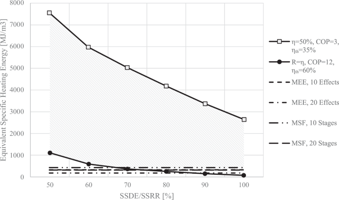
There is a broad operational range for MEFD, due to varying SSDE and SSRR values, COPs, and power plant efficiencies.

An MEFD with a COP of 12, operating with electricity from a power plant with a thermal efficiency of 60%, and with \(\eta =R\ge 70 \%\), has a narrow range of operation where it demonstrates energy merit over 10 effects of the MEE desalination technique. Similarly, for \(\eta =R\ge 65 \%\), the same MEFD shows energy merit over 10 stages of the MSF desalination technique. In order for the MEFD with a COP of 12 to compete with an MEE with 20 effects, the SSDE and the SSRR must be greater than 85%. These factors play a crucial role in reducing the energy consumption of the MEFD and enabling it to be more efficient than the MEE and MSF desalination processes.

The grades of heating energy required for producing electricity in an MEFD and the heating energy extracted from the low-pressure steam turbine for an MEE/MSF are not the same. The heating energy used for producing electrical energy is of higher grade, and therefore the comparison in Fig. 15 is not a complete view. To make a fairer comparison between the MEFD and the MEE, more specific information about the power plant producing the electricity and the steam conditions extracted for running an MEE are required.

For a quick comparison, the lowest temperature of a power plant can be considered as \({T}_{L}=300{K}\) and the highest temperature as \({T}_{H}=1200{K}\). The highest temperature in an MEE and MSF are around 70 °C and 120 °C, respectively²⁸. Assuming a temperature of 120 °C is extracted from the low-pressure section of the steam turbine of a power plant, the MEE is converting the heating energy of 120 °C steam to desalinated water. Therefore, a certain amount of electricity could have potentially been produced if no desalinated water was being produced. Since a certain amount of desalinated water is produced, there is an electrical energy loss due to combining an MEE with a steam power plant.

This problem can be approached from a different perspective as well. A certain power plant uses the higher-grade energy between \({T}_{H}=1200{K}\) and \({T}_{L}=300{K}\) to produce the electrical energy required to operate an MEFD. On the other hand, an MEE utilizes the lower-grade energy contained in the steam with a temperature of \({T}_{H}=343{K}\), while an MSF uses the lower-grade energy contained in the steam with a temperature of \({T}_{H}=393{K}\). The exergy contained in all of these scenarios is calculated and plotted in Fig. 16.

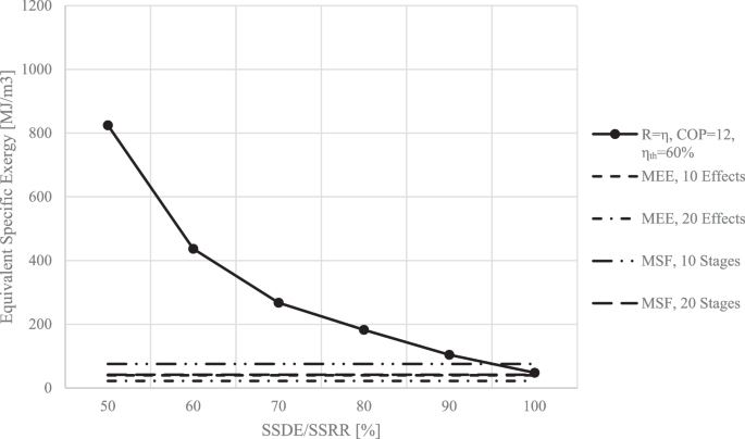
Even under optimal conditions, MEFD with standard feed faces challenges in competing with MEE and MSF.

As observed in Fig. 16, even for the worst-case scenario of an MSF with 10 stages, a well-designed MEFD with a COP of 12 operating on electricity provided from a 60% efficiency power plant has to operate with SSDEs/SSRRs above 95% to be competitive exergy-wise.

It is crucial to acknowledge that while the current study meticulously plans and computes energy consumption and recovery, differences are expected between laboratory and industrial environments. A thorough and intricate energy recovery design, along with real-world factory implementation, is essential to complement this research.